Having fun with rtistry in 280 characters

The practice of creating generative art with the statistical programming language R, also called rtistry, is becoming increasingly popular. However, there aren’t that many resources yet available to learn this practice, and it can sometimes feel to newcomers that its mastery requires writing long and complex programs implementing sophisticated mathematical algorithms.

In part to counteract this impression, and in part just to have fun, I recently wondered what kind of art could be produced with R code that fits entirely into a single tweet, 280 characters:

My challenge was taken up by several people, and here I’d like to show-case some of the interesting examples that were produced. I hope this will be not only entertaining, but also instructive to newcomers of generative art with R. An important aspect of learning how to produce generative art is to take some core concept and see how far you can push it. Change every parameter and see what it does. Change parameters to values you think are crazy. This is much easier with a small code snippet than with a large and complex piece.

To fit a piece of code into 280 characters, we often have to make it quite ugly by deleting all whitespace and violating every style guideline. Here, I’ve taken the liberty to undo these formatting choices to make the code more readable. As a consequence, as posted here, several examples take up more than 280 characters. But in all cases, a fully working example can be produced that fits in its entirety into a single tweet.

Notice: This post contains various code snippets that were not written by me. They are clearly marked, with attribution. All code in this post, including code snippets originally authored by @rtbyts, @1Abstract_1, @KennyVaden, @julian__weis, or myself, has been released under CC0.

Examples using base R

Several examples were proposed with base R. Base R has the advantage that no packages need to be loaded and the core plotting functions are very terse, so it’s possible to pack a lot of logic into 280 characters.

The first example I’ll show was proposed by Torsten Sauer (@rtbyts) in this tweet. I have added a random seed to ensure the code produces the same output every time. Change the random seed to get different versions.

set.seed(66430) # not part of original example

a <- seq(0, pi * 340, length.out = 1000)
r <- seq(0, 14, length.out = 1000)
par(mar = rep(0, 4))
plot(NULL, xlim = c(-9, 9), ylim = c(-9, 9))
points(
  sin(a) * r, cos(a) * r, cex = r * 3, pch = 16,
  col = scales::alpha(sample(rainbow(100)), 0.1)
)

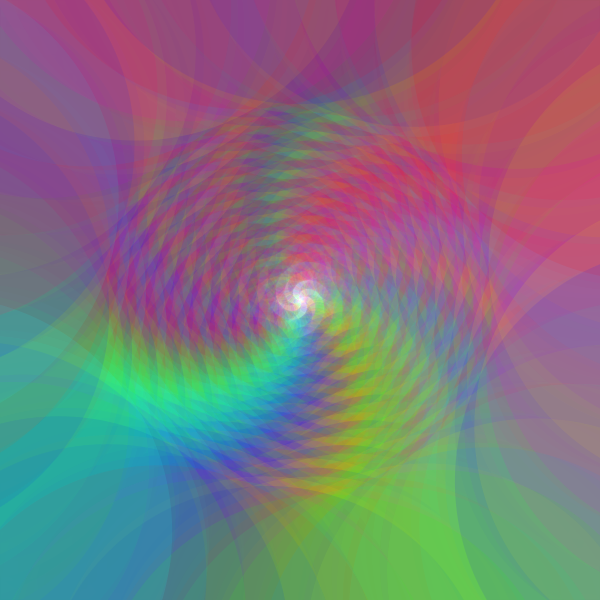
@julian__weis subsequently proposed a modification resulting in an entirely different appearance.

a <- seq(0, pi * 340, length.out = 1000)
r <- seq(0, 14, length.out = 1000)
par(mar = rep(0, 4))
plot(NULL, xlim = c(-40, 40), ylim = c(-40, 40))
points(sin(a) * r, cos(a) * r, cex = 3 * r, pch = 5, col = r)

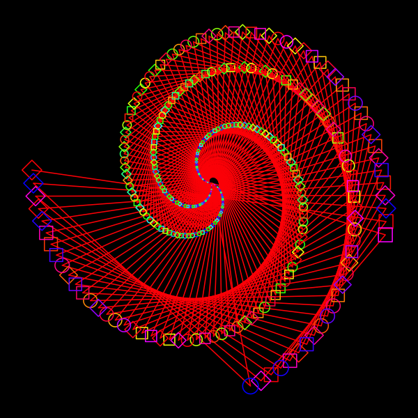
The next example was proposed by @KennyVaden in this tweet. Again I have added a random seed to ensure the code produces the same output every time.

set.seed(12345) # not part of original example

par(mar = rep(.85, 4), bg = 'black')
a = seq(2, 0, length = 100)
n = sample.int(10, 1)
rnd = (a + rep(sample(200, n) * .01, 100)) * pi
plot(
  sin(rnd) * a * 4, cos(rnd) * a * 4, 'o',
  cex = a, pch = 20 + sample.int(3, n * 100, T),
  col = rainbow(120)
)

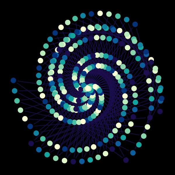
My own take on this idea:

par(mar = rep(.85, 4), bg = 'black')
set.seed(58435)
a = seq(2, 0, length = 100)
n = sample.int(10, 1)
rnd = (a + rep(sample(200, n) * .01, 100)) * pi
plot(
  sin(rnd) * a * 4, cos(rnd) * a * 4, 'b',
  cex=1.5, pch=19,
  col=colorspace::sequential_hcl(10, palette="YlGnBu")
)

Examples using tidyverse packages

Next I’ll show some examples using tidyverse packages and ggplot. These are much more verbose, and yet it’s possible to pack a lot into 280 characters.

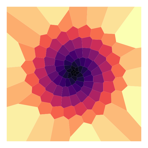
A great concept with many opportunities for subsequent modification was proposed by @1Abstract_1 in this tweet. This piece uses Voronoi tessellation to create a surprisingly complex shape with very little code.

library(tidyverse); library(viridis); library(ggvoronoi)

c <- magma(121)
t <- seq(0, 120, by = 1)
x <- t * cos(t); y <- t * sin(t); p <- data.frame(x, y)

ggplot(p, aes(x, y)) + 
  scale_fill_identity() +
  geom_voronoi(aes(fill = c)) +
  theme_void()

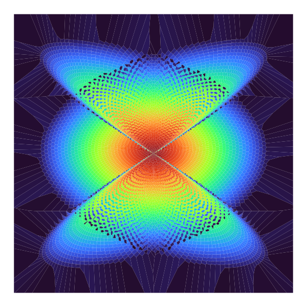
I suggested a variation of this idea here. The main difference is that the Voronoi centers no longer fall onto a simple spiral. I also increased the number of Voronoi centers by two orders of magnitude.

library(tidyverse)

c = rev(viridis::turbo(12345))
t = 0:12344
x = t * cos(3 * t); y = t * sin(2 * t)

ggplot(tibble(x, y), aes(x, y)) + 
  scale_fill_identity() + 
  ggvoronoi::geom_voronoi(aes(fill = c)) + 
  coord_fixed() + 
  theme_void()

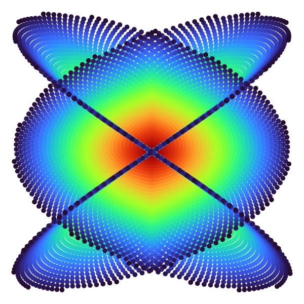
To understand a bit better what is happening here, it’s helpful to plot this as points rather than as Voronoi tessellation. This also yields an interesting artwork in its own right.

library(tidyverse)

c = rev(viridis::turbo(12345))
t = 0:12344
x = t * cos(3 * t); y = t * sin(2 * t)

ggplot(tibble(x, y), aes(x, y)) + 
  scale_color_identity() + 
  geom_point(aes(color = c)) + 
  coord_fixed() +
  theme_void()

Examples without trigonometric functions

All of the examples so far were fundamentally based on using trigonometric functions to create interesting, spiraling patterns. Thus, Torsten Sauer posted:

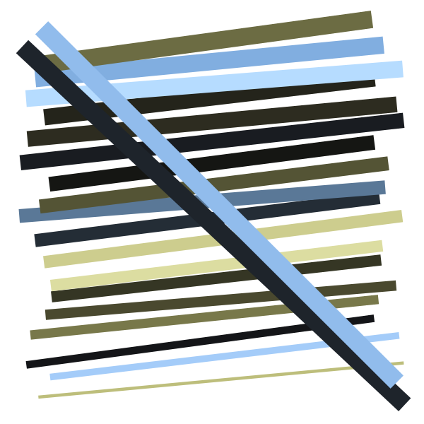
I took him up on the challenge with two pieces. The first one creates a simple line arrangement.

library(tidyverse)

set.seed(6)

tibble(
  x = rep(1:2, each = 20) + .1 * runif(40),
  y = c(0:19, 2:21) %% 20 + .6 * runif(40),
  z = rep(1:20, 2),
  c = sample(colorspace::diverging_hcl(40, palette="Lisbon"), 40)
) |> 
  ggplot(aes(x, y, color = c, group = z, size = x + y)) +
  geom_line() +
  scale_color_identity() +
  cowplot::theme_nothing()

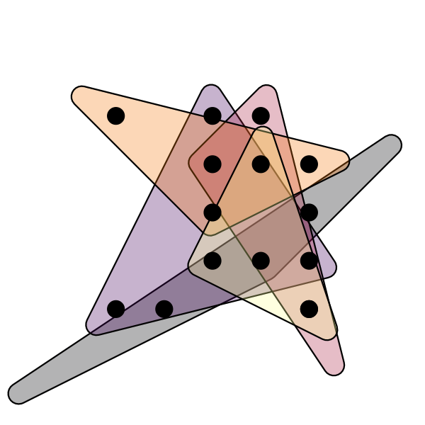
The second one uses geom_mark_hull() from ggforce to create a pattern reminiscent of Dmitri Cherniak’s Ringers.

library(tidyverse)

set.seed(19)

map_dfr(
  letters[2:6],
  ~tibble(x = sample(2:6, 3), y = sample(2:6, 3), z = .x)
) |>
  ggplot(aes(x, y, fill = z)) + 
  ggforce::geom_mark_hull() + 
  geom_point(size = 5) + 
  coord_fixed() + 
  xlim(0, 8) + ylim(0, 8) + 
  scale_fill_viridis_d(option="B") + 
  cowplot::theme_nothing()

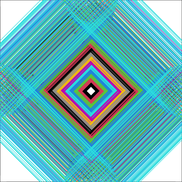
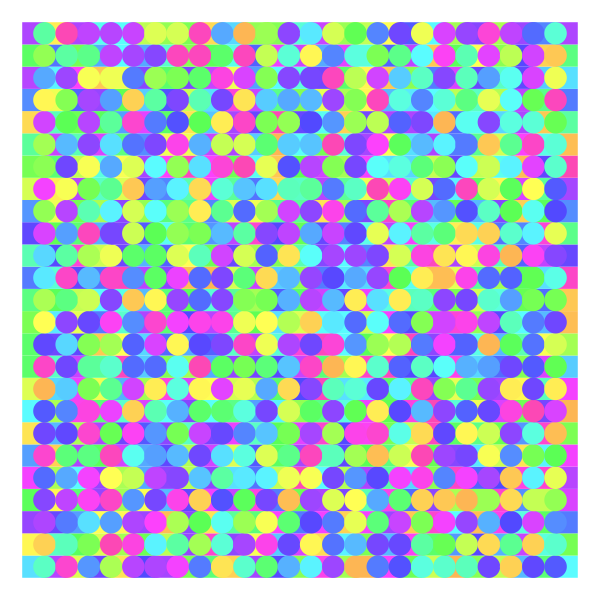
Subsequently, Torsten Sauer himself also posted an example without trigonometric functions:

b <- 25
c <- rainbow(100, 0.6, 1, 0.1, 0.9)
l <- c(1, b + 1)
par(mar = rep(0, 4))
plot(NULL, xlim = l, ylim = l, axes = F)
for(i in seq(b)){
  for(j in seq(b)){
    polygon(
      c(i, i, i + 1, i + 1),
      c(j, j + 1, j + 1, j),
      col = sample(c, 1),
      border = NA
    )
    if (i > 1 & i <= b) 
      points(
        i, j + 0.5, pch = 16, col = sample(c, 1),
        # cex was adjusted to fit the plot size used here;
        # the original value was 5
        cex = 2
      )
  }
}

I hope you’ve found these examples helpful. I encourage you to play around with them and see what happens when you change parameters or colors. Also, I hope I’ll see your contributions to the #rtistry280 hashtag soon.