Probabilistic hatching of polygons
29 November 2021
I have previously discussed techniques to render polygons with a
stippled texture. Here, I want to
build on these earlier ideas to generate a hatched texture. As a
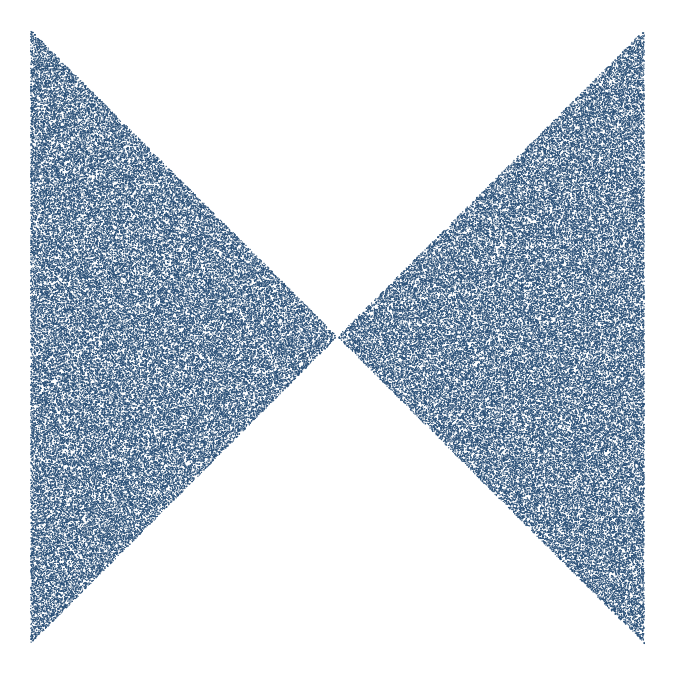
starting point, let’s first review the prior technique. What we did, in
a nutshell, was to generate a cloud of randomly distributed points and
then retain only the ones that lie inside a polygon. To determine
whether a point is inside a polygon boundary or not, we used the R
function sp::point.in.polygon() from the {sp} package. The following
example demonstrates this idea.
library(tidyverse)

# the polygon, two triangles touching in the middle
poly_x <- c(0, 1, 1, 0)
poly_y <- c(0, 1, 0, 1)

# the extent of the initial point cloud
xlim <- c(-.5, 1.5)
ylim <- c(-.5, 1.5)

n <- 1000 # number of points along one dimension
data <- expand_grid(
  # generate uniform grid of points
  x = seq(xlim[1], xlim[2], length.out = n),
  y = seq(ylim[1], ylim[2], length.out = n),
) %>%
  mutate(
    # jitter the points a little
    x = x + rnorm(n(), sd = 0.01),
    y = y + rnorm(n(), sd = 0.01),
    # test whether each point is inside the polygon or not
    interior = (sp::point.in.polygon(x, y, poly_x, poly_y) == 1)
  ) %>%
  filter(interior)

ggplot(data, aes(x, y)) +
  geom_point(size = 0.3, stroke = 0, color = "steelblue4") +
  coord_fixed() +
  theme_void()
Now, we’d like to apply a hatching effect rather than a stippling effect when rendering this polygon. To hatch, we need to draw line segments instead of points. A simple way to do this is to pair every random point in the previous example with a second point and draw a line segment between the two. To ensure that the line segments all have approximately the same length and point in all possible directions, we will place the second points randomly on circles around the first points, using circle radii drawn from a normal distribution.
make_hatch_1 <- function(radius = 0.1, radius_sd = 0.01, n = 1000) {
  expand_grid(
    x = seq(xlim[1], xlim[2], length.out = n),
    y = seq(ylim[1], ylim[2], length.out = n),
  ) %>%
    mutate(
      x = x + rnorm(n(), sd = 0.01),
      y = y + rnorm(n(), sd = 0.01),
      # randomly generate radius and angle
      r = rnorm(n(), mean = radius, sd = radius_sd),
      theta = runif(n(), max = 2 * pi),
      # place segment end points on circles around start points
      xend = x + r * cos(theta),
      yend = y + r * sin(theta),
      # test whether both start and end points are in polygon
      interior = (sp::point.in.polygon(x, y, poly_x, poly_y) == 1) &
        (sp::point.in.polygon(xend, yend, poly_x, poly_y))
    ) %>%
    filter(interior)
}

make_hatch_1() %>%
  ggplot(aes(x, y)) +
  geom_segment(
    aes(xend = xend, yend = yend),
    size = 0.05, alpha = 0.08, color = "steelblue4"
  ) +
  coord_fixed() +
  theme_void()
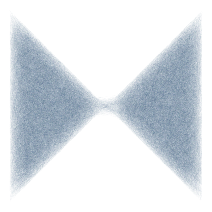
I have encapsulated the hatching logic in the function make_hatch_1()
so we can play around with parameters and see what happens. By changing
the mean and standard deviation of the distribution from which we draw
radii, we can create different flavors of texture. For example, short
radii create a felt-like texture.
make_hatch_1(radius = 0.02, radius_sd = 0.01) %>%
  ggplot(aes(x, y)) +
  geom_segment(aes(xend = xend, yend = yend), size = 0.2, alpha = 0.15, color = "steelblue4") +
  coord_fixed() +
  theme_void()

We can add additional complexity by changing how we generate the initial
dot distribution. For example, instead of distributing dots uniformly
over the canvas, we can place them in clusters, and also give different
clusters different colors. This creates interesting gradient effects.
The following function make_hatch_2() implements this idea. It also
has a number of additional options we will explore momentarily.
make_hatch_2 <- function(radius = 0.1, radius_sd = 0.02, min = 0, max = 2*pi,
                         size = 0.15, alpha = 0.1, filter_endpoints = TRUE,
                         n = 50000) {
  tibble(
    # the initial point distribution now consists of three Gaussian clouds
    x = c(rnorm(n, mean = 0.7, sd = 0.2), rnorm(n, mean = 0.2, sd = 0.2), rnorm(n, mean = 0.4, sd = 0.3)),
    y = c(rnorm(n, mean = 0.85, sd = 0.2), rnorm(n, mean = 0.95, sd = 0.2), rnorm(n, mean = 0.2, sd = 0.3))
  ) %>%
    mutate(
      r = rnorm(n(), mean = radius, sd = radius_sd),
      theta = runif(n(), min = min, max = max),
      xend = x + r * cos(theta),
      yend = y + r * sin(theta),
      interior = (sp::point.in.polygon(x, y, poly_y, poly_x) == 1) &
        (!filter_endpoints | sp::point.in.polygon(xend, yend, poly_y, poly_x)),
      # colors for the three Gaussian clouds
      color = rep(c("goldenrod3", "coral4", "olivedrab"), each = n),
      alpha = alpha,
      size = size
    ) %>%
    filter(interior)
}

# encapsulate plotting in a function, for simplicity of later code
paint <- function(data) {
  ggplot(data, aes(x, y, color = color, size = size, alpha = alpha)) +
    geom_segment(aes(xend = xend, yend = yend)) +
    scale_color_identity(aesthetics = c("color", "size", "alpha")) +
    coord_fixed() +
    theme_void()
}

data1 <- make_hatch_1(radius = 0.02, radius_sd = 0.01) %>%
  mutate(
    color = "steelblue4",
    alpha = 0.15,
    size = 0.2
  )

# combine the two hatch patterns and plot
rbind(data1, make_hatch_2()) %>%
  paint()
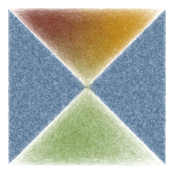
I am showing here both the original technique that uses a uniform point distribution (blue triangles) and the modified technique that uses a clustered point distribution (red/orange/green triangles). In this way, you can see their different appearance side-by-side.
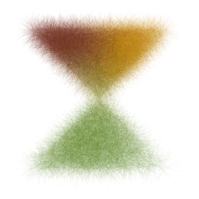
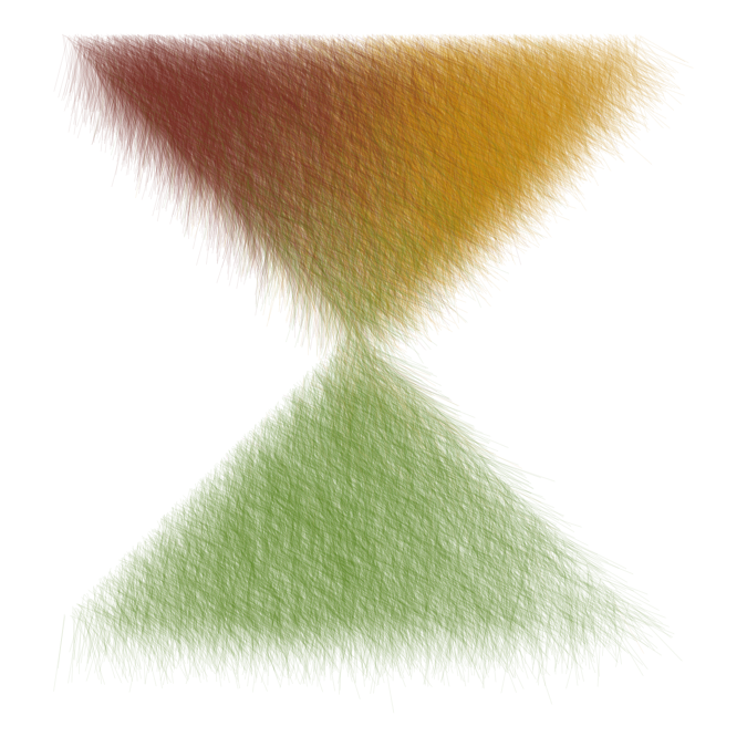
In the above hatching examples, we have only retained segments if both
end points are fully contained within the polygon. If we loosen this
restriction, so that, for example, only the first point is required to
fall inside the polygon, we can generate shapes with rough borders. To
do so we set filter_endpoints = FALSE in make_hatch_2(). We also
remove the blue triangles so you can better see the polygon boundaries.
make_hatch_2(filter_endpoints = FALSE) %>%
  paint()
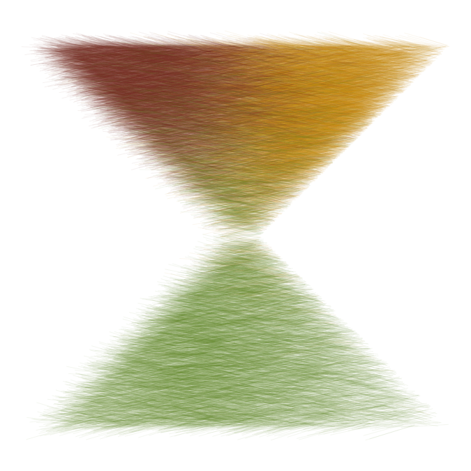
We can also constrain the angles at which we draw line segments. For example, we could use mostly horizontal line segments pointing to the left (angles near 180 degrees). This creates a fur-like texture.
make_hatch_2(filter_endpoints = FALSE, min = 0.9*pi, max = 1.1*pi) %>%
  paint()
Or we could use line segments pointing mostly down and/or to the right. This creates a texture that looks almost like stone.
make_hatch_2(filter_endpoints = FALSE, min = 1.4*pi, max = 1.9*pi) %>%
  paint()
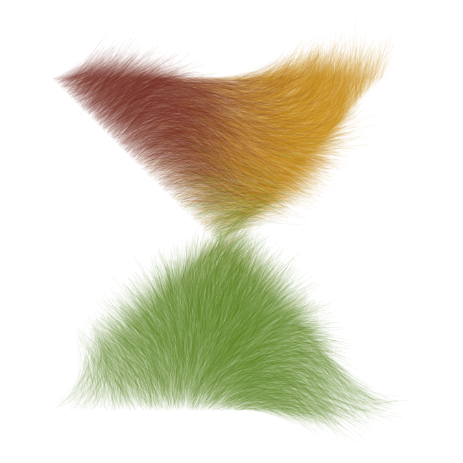
We can add further variation by changing the direction of the line
segments across the canvas, for example based on Perlin noise. This
requires the gen_perlin() function from the {ambient} package. The
result looks like hair (if you ignore the green color).
make_hatch_3 <- function(noise_fun, radius = 0.08, radius_sd = 0.03,
                         size = 0.15, alpha = 0.1, n = 50000) {
  tibble(
    x = c(rnorm(n, mean = 0.7, sd = 0.2), rnorm(n, mean = 0.2, sd = 0.2), rnorm(n, mean = 0.5, sd = 0.2)),
    y = c(rnorm(n, mean = 0.85, sd = 0.2), rnorm(n, mean = 0.95, sd = 0.2), rnorm(n, mean = 0.2, sd = 0.2))
  ) %>%
    mutate(
      noise = noise_fun(x, y),
      r = rnorm(n(), mean = radius, sd = radius_sd),
      theta = runif(n(), min = noise * pi, max = (noise + 0.2) * pi),
      xend = x + r * cos(theta),
      yend = y + r * sin(theta),
      interior = (sp::point.in.polygon(x, y, poly_y, poly_x) == 1),
      color = rep(c("goldenrod3", "coral4", "olivedrab"), each = n),
      alpha = alpha,
      size = size
    ) %>%
    select(-noise) %>%
    filter(interior)
}

set.seed(3557)
make_hatch_3(
  noise = function(x, y) ambient::gen_perlin(x, y, frequency = 1.8)
) %>%
  paint()
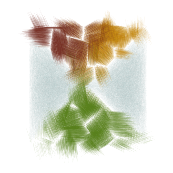
Finally, let’s use some Worley noise and bring back the left and right triangle, but in a lighter color.
set.seed(3590)

make_hatch_1(radius = 0.2, radius_sd = 0.01, n = 500) %>%
  mutate(
    color = "azure3",
    alpha = 0.1,
    size = 0.1
  ) %>%
  rbind(
    make_hatch_3(
      noise = function(x, y) noise = ambient::gen_worley(x, y, frequency = 7)
    )
  ) %>%
  paint()
As you can see, the mechanism described in this post can generate a wide range of different textures and polygon boundaries. We have created textures that look like felt, fur, stone, or hair. I hope you will find these ideas useful in your own explorations of generative art.