Probabilistic stippling of polygons
08 November 2021
In a previous post, I used sigmoidal functions to generate horizontal stripes of colored dots that would blend into each other. If you have read that post, you may have wondered whether a similar effect can be obtained for more complicated shapes. The short answer is yes. In fact, I’m aware of two different approaches, and I will describe both here. The first is coded from scratch and doesn’t require any kind of support library, but is limited to convex polygons. The second is more general but requires access to a library that can test whether a given point lies inside a polygon.
The first approach uses sigmoidal functions as before but applies them along arbitrary edges in 2D space. This is quite straightforward with a little bit of vector calculus. The core concept we need is the scalar rejection, which is the orthogonal distance from one vector to another. We can use it to calculate the distance of a point to an edge, and then feed that distance into our sigmoidal function as before. The following example demonstrates this idea for a single diagonal edge.
library(tidyverse)

sigmoid <- function(x, x1 = 0, slope = 1) {
  1 / (1 + exp(-100*slope * (x - x1)))
}

# distance of (x0, y0) to the line defined by (x1, y1) to (x2, y2)
vector_rejection <- function(x0, y0, x1, y1, x2, y2) {
  dx2 <- x2 - x1
  dx0 <- x0 - x1
  dy2 <- y2 - y1
  dy0 <- y0 - y1

  (dx0*dy2 - dy0*dx2) / sqrt(dx2^2 + dy2^2)
}

n <- 200  # number of dots along one dimension
sd <- 0.005  # amount of noise applied to x/y positions of points

tibble( # create noisy grid of points
  x = rep((1:n)/n, n) + rnorm(n*n, sd = sd),
  y = rep((1:n)/n, each = n) + rnorm(n*n, sd = sd)
) %>%
  mutate( # determine whether points should be included or excluded
    prob = sigmoid(vector_rejection(x, y, 0.3, 0.8, 0.7, 0.2), slope = 0.5),
    include = runif(n()) < prob # include points based on probability value
  ) %>%
  filter(include == TRUE) %>%
  ggplot(aes(x, y)) +
  geom_point(size = 0.2) +
  annotate("point", x = c(.3, .7), y = c(.8, .2), color = "red", size = 4) +
  annotate("segment", x = .3, y = .8, xend = .7, yend = .2, color = "red", size = 1.5) +
  coord_fixed(xlim = c(0, 1), ylim = c(0, 1)) +
  theme_void()
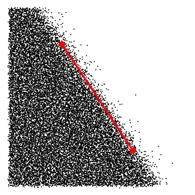
The two connected red dots highlight the line segment that was used to create the boundary between the area with points and the area without.
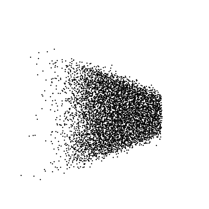
We can extend this concept to arbitrary convex polygons by calculating a sigmoidal function for each polygon boundary and then multiplying all these functions together. One advantage of this method is that it enables us to define different amounts of jitter for the different polygon edges. For example, here the right edge is particularly sharp and the left edge is particularly blurry.
# Calculate the inclusion probability for an arbitrary convex polygon.
# The polygon boundary is defined by the vectors x and y, and
# the points for which the probability is calculated are given
# by x0 and y0.
poly_prob <- function(x0, y0, x, y, slope = 1) {
  x1 <- x
  y1 <- y
  x2 <- lead(x1, default = x1[1])
  y2 <- lead(y1, default = y1[1])
  slope <- rep_len(slope, length(x1))

  prob <- rep_len(1, length(x0))
  for (i in seq_along(x1)) {
    p <- sigmoid(vector_rejection(x0, y0, x1[i], y1[i], x2[i], y2[i]), slope = slope[i])
    prob <- prob * p
  }
  prob
}

# x and y coordinates for the enclosing polygon
poly_x <- c(0.4, 0.8, 0.8, 0.4)
poly_y <- c(0.7, 0.55, 0.35, 0.2)
# slope parameters for each polygon edge
slope <- c(1, 10, 1, .2)

tibble( # create noisy grid of points
  x = rep((1:n)/n, n) + rnorm(n*n, sd = sd),
  y = rep((1:n)/n, each = n) + rnorm(n*n, sd = sd)
) %>%
  mutate( # determine whether points should be included or excluded
    prob = poly_prob(x, y, poly_x, poly_y, slope),
    include = runif(n()) < prob
  ) %>%
  filter(include == TRUE) %>%
  ggplot(aes(x, y)) +
  geom_point(size = 0.2) +
  coord_fixed(xlim = c(0, 1), ylim = c(0, 1)) +
  theme_void()
The disadvantage of this approach is that it is strictly limited to convex polygons, because each sigmoidal function segments the entire 2D plane into two parts separated by a straight line of infinite length. For convex polygons, these lines will never intersect with other parts of the polygon, but for arbitrary shapes this is not guaranteed.
The second approach retires the sigmoidal functions. Instead it takes a
cloud of points and clips it to a polygon. This allows for arbitrary,
non-convex shapes, and it works well as long as we have access to a
function that can determine whether a point is inside a polygon or not.
In R, the {sp} package provides a function point.in.polygon() that
does exactly that, and we will use it going forward.
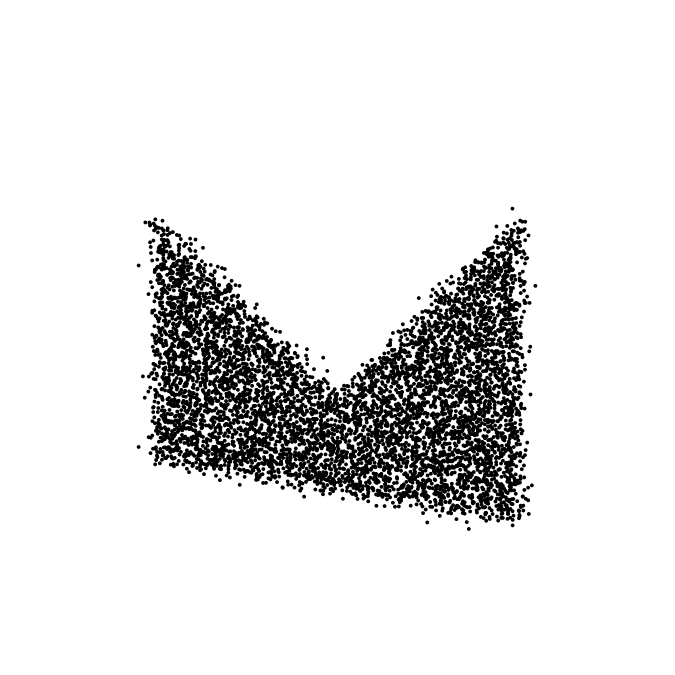
However, clipping points to a polygon creates hard boundaries, and we wanted to have smooth boundaries where points slowly fade out. The solution is to generate a regular grid of points, filter out all the points that are interior (or exterior) to a given polygon, and then apply Gaussian noise to the point coordinates to create texture and smooth polygon edges.
# x and y coordinates for the enclosing polygon
poly_x <- c(0.2, 0.5, 0.8, 0.8, 0.2)
poly_y <- c(0.7, 0.4, 0.7, 0.2, 0.3)

n <- 200  # number of dots along one dimension
sd <- 0.01  # amount of noise applied to x/y positions of points

tibble( # create regular grid of points without noise
  x = rep((1:n)/n, n),
  y = rep((1:n)/n, each = n)
) %>%
  mutate(
    # determine whether points are interior or exterior
    # to the polygon; a value of 1 means strictly interior point
    interior = sp::point.in.polygon(x, y, poly_x, poly_y) == 1
  ) %>%
  filter(interior == TRUE) %>%
  mutate( # add noise to the point positions
    x = x + rnorm(n(), sd = sd),
    y = y + rnorm(n(), sd = sd)
  ) %>%
  ggplot(aes(x, y)) +
  geom_point(size = 0.2) +
  coord_fixed(xlim = c(0, 1), ylim = c(0, 1)) +
  theme_void()
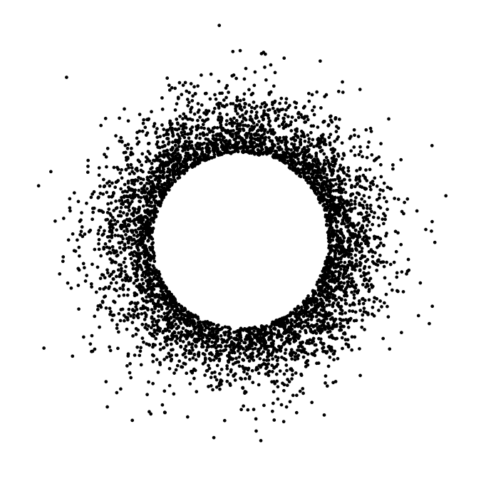
Second, we can create a noisy point cloud first and then clip to the interior or exterior of a polygon. As mentioned above, this creates a sharp polygon edge. But if we retain only the points exterior to the polygon we achieve a nice shadow-like effect. I like to do this with Gaussian noise clipped to a circle.
# x and y coordinates of circle
poly_x <- 0.2*cos(seq(0, 2*pi, length.out = 100)) + 0.5
poly_y <- 0.2*sin(seq(0, 2*pi, length.out = 100)) + 0.5

n <- 20000  # total number of dots created
sd <- 0.12  # amount of noise

tibble(
  x = rnorm(n, mean = 0.5, sd = sd),
  y = rnorm(n, mean = 0.5, sd = sd)
) %>%
  mutate(
    # a value of 1 means strictly interior point
    interior = sp::point.in.polygon(x, y, poly_x, poly_y) == 1
  ) %>%
  filter(interior == FALSE) %>%
  ggplot(aes(x, y)) + geom_point(size = 0.4) +
  coord_fixed(xlim = c(0, 1), ylim = c(0, 1)) +
  theme_void()
Now we will combine these techniques to create an actual artwork. We begin by encapsulating the above ideas into reusable functions.
# sets the resolution of the final render; higher numbers mean better resolution
scale <- 2

# function that creates a circle with exterior shadow
render_circle <- function(x = 0.5, y = 0.5, r = 0.1, n = r*r*500000*scale*scale, sd = 0.5*r, color = "#254F82") {
  poly_x <- r*cos(seq(0, 2*pi, length.out = 100)) + x
  poly_y <- r*sin(seq(0, 2*pi, length.out = 100)) + y

  tibble(
    x = rnorm(n, mean = x, sd = sd),
    y = rnorm(n, mean = y, sd = sd),
    color = color
  ) %>%
    mutate(
      interior = sp::point.in.polygon(x, y, poly_x, poly_y) == 1
    ) %>%
    filter(interior == FALSE) %>%
    select(x, y, color)
}

# function that creates a filled rectangle with soft edges
render_rect <- function(x = 0.5, y = 0.5, width = 0.2, height = 0.2, n = 200*scale, sd = 0.005, color = "#254F82", xlim = c(-0.1, 1.1), ylim = c(-0.1, 1.1)) {
  poly_x <- c(x - width/2, x + width/2, x + width/2, x - width/2)
  poly_y <- c(y + height/2, y + height/2, y - height/2, y - height/2)

  expand_grid(
    x = seq(xlim[1], xlim[2], length.out = n),
    y = seq(ylim[1], ylim[2], length.out = n)
  ) %>%
    mutate(
      interior = sp::point.in.polygon(x, y, poly_x, poly_y) == 1
    ) %>%
    filter(interior == TRUE) %>%
    mutate(
      x = x + rnorm(n(), sd = sd),
      y = y + rnorm(n(), sd = sd),
      color = color
    ) %>%
    select(x, y, color)
}

# function to render the final artwork
paint <- function(data, size = 0.7/scale) {
  ggplot(data, aes(x, y, color = color, group = 1)) +
  geom_point(size = size, stroke = 0) +
  scale_color_identity() +
  coord_fixed(xlim = c(0, 1), ylim = c(0, 1)) +
  theme_void() +
  theme(
    plot.background = element_rect(fill = "#FEF6E6", color = NA)
  )
}
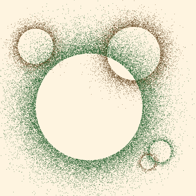
Now, let’s use these functions to create a few circles of different sizes and colors.
make_circles <- function() {
  tibble(
    x = c(.15, .7, .45, .85, .78),
    y = c(.79, .75, .45, .2, .14),
    r = c(.1, .15, .3, .06, .04),
    color = c("#674108", "#674108", "#056023", "#056023", "#674108")
  ) %>%
    mutate(
      data = pmap(list(x, y, r, color), function(x, y, r, col)
        render_circle(x, y, r, color = col)
      )
    ) %>%
    select(-r, -x, -y, -color) %>%
    unnest(data)
}

paint(make_circles())
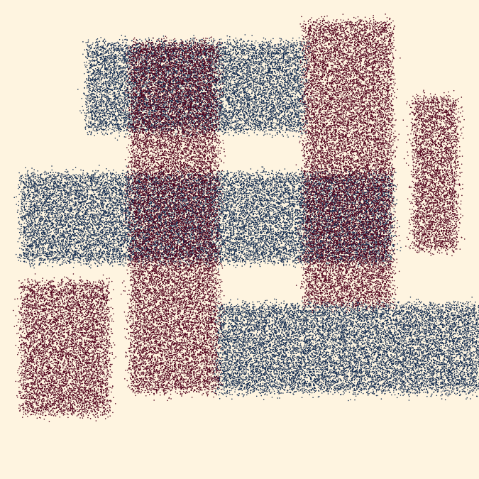
And simiarly, let’s also create a few rectangles of different sizes and colors.
make_rects <- function() {
  tibble(
    x = c(.4, .425, .75, .35, .75, .1, .95),
    y = c(.85, .55, .25, .55, .675, .25, .65),
    w = c(.5, .85, .6, .2, .2, .2, .1),
    h = c(.2, .2, .2, .8, .65, .3, .35),
    color = c(rep("#133861", 3), rep("#640723", 4))
  )%>%
    mutate(
      data = pmap(list(x, y, w, h, color), function(x, y, w, h, col)
        render_rect(x, y, color = col, width = w, height = h, sd = 0.008)
      )
    ) %>%
    select(-w, -h, -x, -y, -color) %>%
    unnest(data)
}

paint(make_rects())
Finally, we combine these two pieces by plotting the rectangles on top
of the circles. We also dramatically increase the resolution (by
increasing scale) to obtain a more refined result.
scale <- 30

rbind(
  make_circles(),
  make_rects()
) %>%
  paint()
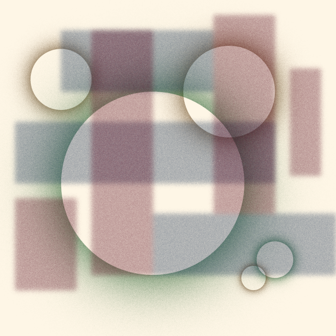
This artwork was inspired in part by Circles of Dust posted on Reddit. I have no information about how Circles of Dust was created, but I believe it uses similar techniques to the ones I have discussed here.