Raytraced 3D t-SNE sculptures

The t-SNE method is conventionally used to project high-dimensional data into two dimensions, but we can also use it to project into three dimensions. This generates sculptures that we can visualize using some 3D rendering approach, such as raytracing. Here, I will describe the basic process for doing this in R, using the rayrender package. The code will be quite similar to earlier code I posted to make 2D t-SNE art.

First we load the required packages.

library(tidyverse)
library(Rtsne)
library(rayrender)

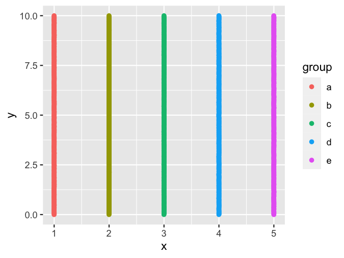
Next we define a function that generates our input dataset. This can be in two dimensions even if the t-SNE output will be in three dimensions. For simplicity, I’m just creating some vertical stripes. You can use other initial arrangements, but stripes go surprisingly far.

setup_coords <- function(groups = 5, n = 400, sd = .001) {
  tibble(
    x = rep(1:groups, each = n) + rnorm(groups*n, sd = sd),
    y = rep(seq(from = 0, to = 10, length.out = n), groups) + 
      rnorm(groups*n, sd = sd),
    group = rep(letters[1:groups], each = n)
  )
}

setup_coords() %>%
  ggplot(aes(x, y, color = group)) + geom_point()

Next, we run this input data through the t-SNE algorithm.

do_tsne <- function(coords, perplexity = 3) {
  tsne_fit <- coords %>%
    select(x, y) %>%
    scale() %>%
    Rtsne(dims = 3, perplexity = perplexity, max_iter = 500, check_duplicates = FALSE)
  
    tsne_fit$Y %>%
      scale() %>%
      as.data.frame() %>%
      cbind(select(coords, -x, -y)) %>%
      rename(x = V1, y = V2, z = V3)
}

set.seed(68440) # pick an arbitrary random seed for reproducibility
tsne_coords <- setup_coords() %>%
  do_tsne() 

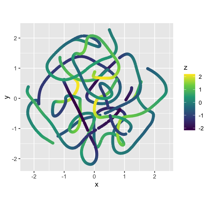
To get a sense of what the result is, we can visualize the result in two dimensions, using color for depth.

ggplot(tsne_coords, aes(x, y, color = z)) + 
  geom_point() + 
  scale_color_viridis_c() +
  coord_fixed()

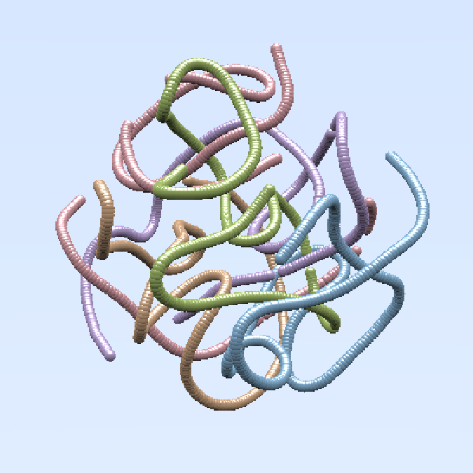
Now let’s go into the third dimension. We simply place a sphere at the location of each point in the dataset we just created. To make it a little more interesting, we use different colors for the five different stripes we generated as input.

colors <- c(a = '#5796CD', b = '#A182CF', c = '#C18355', d = '#CF7781', e = '#7A9C38')

spheres <- pmap_dfr(
  list(tsne_coords$x, tsne_coords$y, tsne_coords$z, tsne_coords$group),
  function(x, y, z, g) {
    sphere(
      x, y, z, radius = 0.07,
      material = glossy(color = colors[g], reflectance = 0.1)
    )
  })

Let’s do a quick render of the sculpture so far.

render_preview(spheres, lookfrom = c(6, 1.5, 13), fov = 23)

Here, lookfrom is the position of the camera, and fov stands for “field of view”. The field of view is an angle that determines how much of the scene you can see. Imagine the difference between a telescope and a wide-angle lense in photography. You can play around with different fov values to make the sculpture appear closer to the camera or further away.

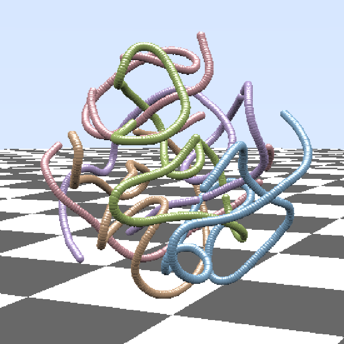
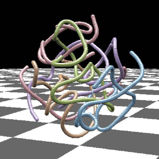
Next we make the scene a little more interesting by adding a checkerboard floor. For now, we still visualize with the quick preview.

scene <- generate_ground(depth = -2.5, material = diffuse(checkercolor = "grey20")) %>%
  add_object(spheres)

render_preview(scene, lookfrom = c(6, 1.5, 13), fov = 23)

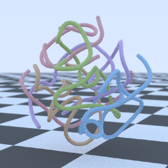
We can raytrace this scene but the result doesn’t look so impressive. That’s because there’s a lot of ambient blue light that causes everything to look washed out and blue.

render_scene(scene, lookfrom = c(6, 1.5, 13), fov = 23)

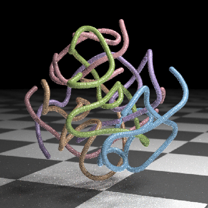
Instead, we will add two explicit light sources. This causes rayrender to turn off the ambient light. The preview doesn’t look that different, other than that the sky is now black rather than blue.

scene <- generate_ground(depth = -2.5, material = diffuse(checkercolor = "grey20")) %>%
  add_object(spheres) %>%
  add_object(sphere(x = 8, y = 7, z = 4, radius = 2, material=light(intensity = 20))) %>%
  add_object(sphere(x = 3, y = 10, z = -4, radius = 2, material=light(intensity = 20)))

render_preview(scene, lookfrom = c(6, 1.5, 13), fov = 23)

But when we ray trace, we see that the result is now dramatically different.

render_scene(scene, lookfrom = c(6, 1.5, 13), fov = 23)

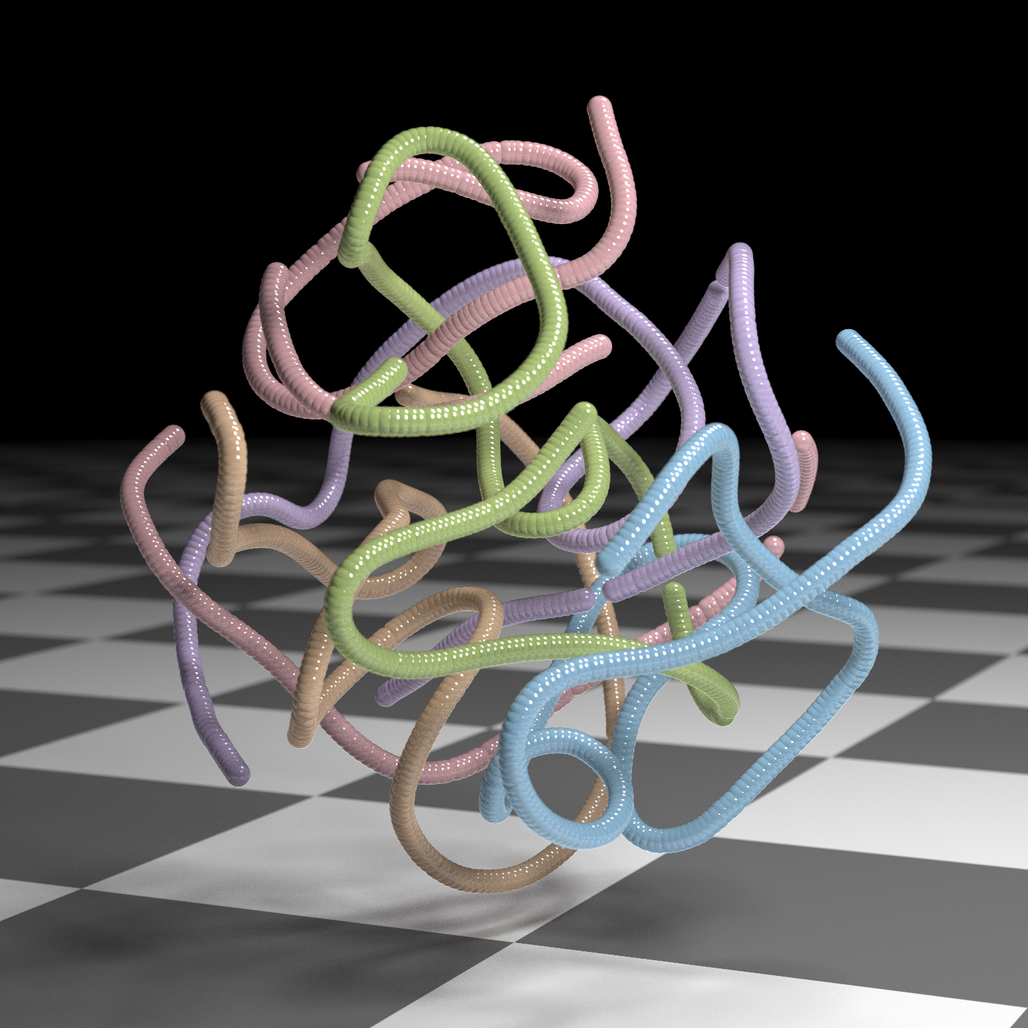
Finally, for photorealistic rendering, we need to up the quality parameters. We set clamp_value = 10 to remove bright spots of light, samples = 2000 and min_variance = 5e-6 to do more extensive sampling for each pixel, and width = 1500 and height = 1500 to render a higher-resolution image. The following code may take 30 minutes or more to run, so be aware that this is not code to be used interactively. Rendering high-resolution, photorealistic images takes a lot of compute power.

render_scene(
  scene, lookfrom = c(6, 1.5, 13), fov = 23, clamp_value = 10,
  width = 1500, height = 1500, samples = 2000,
  min_variance = 5e-6,
  filename = "tSNE-3D"
)

You can see my own set of 3D sculptures in my series Nonlinear Dimension Reduction. Every piece in that series was created using code very similar to what I’ve shown here. I just played around with different input datasets, different t-SNE parameters, different materials, and different lighting setups.