Writing a blogdown post for the ages

The R package blogdown has become a widely popular solution to setting up personal blogs. It makes it super easy to set up quite elaborate websites, and to write posts that contain R code, generated output and figures, footnotes, figure references, and math.¹ However, one problem with blogdown is that it likes to re-knit .Rmd files.² This may be fine if you’re just starting out with your site or if your posts generally don’t contain any sophisticated R code, but in a long-standing blog you’ll eventually run into trouble. First, re-knitting hundreds of posts may be quite slow. And second, if you’ve got a bunch of old posts chances are some will not knit anymore, and then you may have got a serious problem with no simple solution.

This problem has been recognized for a while, and the proposed solution is usually to knit only on demand. See e.g. here. The experimental hugodown package likewise aims to limit any unnecessary re-knitting. Here, I’m taking a different approach. My perspective is that I want to be able to re-knit any time without worrying that I’ll destroy anything of value, and I also want to be able to add code and output to posts containing prior code that doesn’t run anymore today.

My approach is to copy the knitted markdown code and output back into the .Rmd file. This requires some amount of manual work, but it’s not that bad, and I value the benefits I get from this approach. Maybe at some point somebody will write a package that can automate this process.

I do not necessarily recommend the approach I’m taking here. This post is mostly for my own purposes, so I can retrace my steps in the future. If you want to see the source code resulting from this process, you can check out the source for this post on github.

To provide an example scenario, I include here one chunk of R code that generates a figure. This code has various features that will likely generate issues in the future or in a blog with many posts:

• It depends on a bunch of packages, including one only available from github.
• It uses various fonts that need to be installed locally.
• It is slow to render.

So it is critical that we can capture the output and don’t ever have to re-render it again.

Here is the example:

library(tidyverse)
library(cowplot)
library(colorspace)
library(sf) 
library(ggtext)

# attach data set, requires practicalgg package
# remotes::install_github("wilkelab/practicalgg")
data(texas_income, package = "practicalgg")

ggplot(texas_income, aes(fill = estimate)) + 
  geom_sf(color = "white") +
  coord_sf(xlim = c(538250, 2125629), crs = 3083) +
  scale_fill_continuous_sequential(
    palette = "Blues", rev = TRUE,
    na.value = "grey60",
    name = "annual median income (USD)",
    limits = c(18000, 90000),
    breaks = 20000*c(1:4),
    labels = c("$20,000", "$40,000", "$60,000", "$80,000"),
    guide = guide_colorbar(
      direction = "horizontal",
      label.position = "bottom",
      title.position = "top",
      barwidth = grid::unit(3.0, "in"),
      barheight = grid::unit(0.2, "in")
    )
  ) +
  labs(caption = "
<span style='font-family: \"Font Awesome 5 Brands\"'>&#xf099;</span>
@clauswilke<br>
<span style='font-family: \"Font Awesome 5 Free Solid\"'>&#xf781;</span>
clauswilke.com
") +
  theme_map(12, font_family = "Myriad Pro") +
  theme(
    legend.title.align = 0.5,
    legend.text.align = 0.5,
    legend.justification = c(0, 0),
    legend.position = c(0.02, 0.1),
    plot.caption = element_markdown()
  )

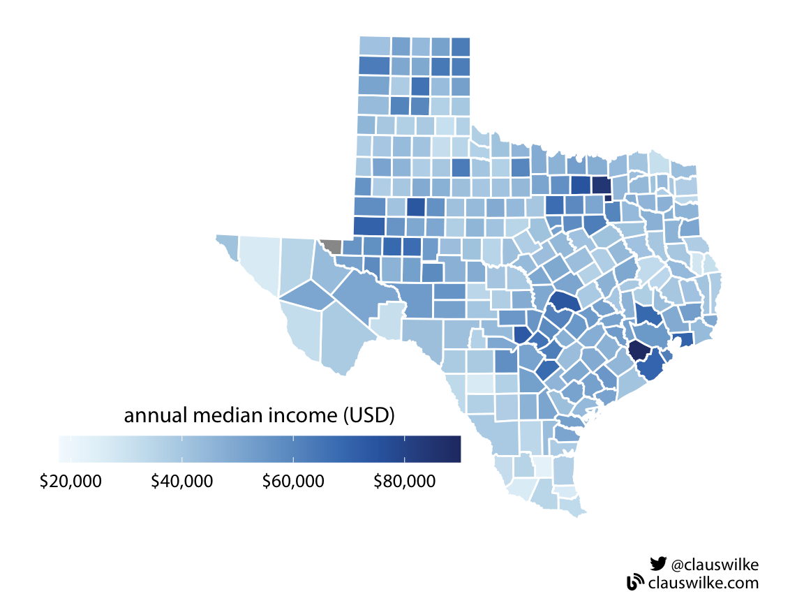
Figure 1: Median annual income in Texas counties. Figure redrawn from: Wilke (2019) Fundamentals of Data Visualization, Chapter 4.

Next I’ll provide the exact recipe I follow to capture the output from such code.

1. At the top of your .Rmd file, add an R chunk containing the following:

   ```{r echo = FALSE}
   knitr::opts_chunk$set(fig.retina = 2)
   ```

   This will ensure that figures are rendered in high quality. Set echo = FALSE for this chunk so the code isn’t included in the rendered output.

2. Stop the blogdown server with blogdown::stop_server(). We don’t want the server to try to create blog posts out of the intermediate files we’ll be creating.

3. Add the following to the yaml section of your post:

   output:
     html_document:
       keep_md: yes
   

   If you want to use bookdown-style automated figure references, use this snippet instead:

   output:
     bookdown::html_document2:
       keep_md: yes
   

   This requires the bookdown package to be installed.

4. Knit your post. You will end up with a new file index.md and a new folder called index_files. The former contains the markdown code that knitr has generated and the latter contains any generated figures.

5. Now you want to copy the generated code and output chunks from index.md back into index.Rmd. For each code chunk in your .Rmd file, there will be one or more markdown chunks, which are fenced with ```r ...```. There will also be markdown or HTML code to include any generated figures. Place all of this material after the respective code chunk from which it originated, but do not delete the original code chunk. We want to keep the original code chunks around in case we do want to re-run some of the R code again in the future, e.g. if the post needs an update.

6. Next, you need to move the generated figures into a safe location. This ensures that they won’t be deleted when blogdown rebuilds the site the next time. I simply move the folder index_files/figure-html to figure-html.

7. Edit figure links to reflect the move from the previous step. Figure links may be included either as markdown links, such as ![](index_files/figure-html/map-Texas-income-1.png), or as html links, such as <img src="/blog/2020-09-08-a-blogdown-post-for-the-ages/index_files/figure-html/map-Texas-income-1.png" .... Which is the case depends on the exact chunk options you used to generate the figure. In either case, delete index_files/ from all figure links.

8. Delete the file index.md.

9. Remove or comment out the output: block you added under step 3.

10. Add the following line to the code chunk added under step 1:
    

    knitr::opts_chunk$set(echo = FALSE, eval = FALSE)
    

    This turns off all the R Markdown chunks in your post.

11. Restart the blogdown server with blogdown::serve_site().

This may seem like a lot of steps and a lot of fiddling, but it’s really not that bad once you get the hang of it. Most blog posts, even elaborate ones, don’t have that many code chunks or figures, and manually copying and adjusting the markdown code takes much less time than writing the blog post in the first place.

In the future, if you need to update your post, you can either re-run all code by commenting out the line you added in step 10, or you can selectively turn on individual R chunks by setting their echo and eval options to TRUE. Then you repeat steps 1 through 11, but copying only whichever output needs to be newly copied over. At the end make sure you disable all R chunks once again.